今回は、話題の画像生成AI「Stable Diffusion」を、「stable_diffusion.ipynb - Colaboratory - Google」のPythonコードの解説と、説明文の日本語翻訳で紹介したいと思います。
Stable Diffusion とは、テキストを入力するとそれに沿った画像を生成してくれるAIモデルで、Colaboratory というオンラインのプログラミング環境で簡単に実行できます。
Stable Diffusion のコードの解説を読んで理解することで、画像生成AIの仕組みやプログラミングスキルを学ぶことができます。
この記事では、Stable Diffusionのコードの概要と詳細、実行と結果の紹介を行います。
画像生成AIに興味がある方や、プログラミングのスキルアップを目指す方は、ぜひ最後までお読みください。
- Stable DiffusionのColaboratory環境を準備
- Stable Diffusionの説明文を日本語化
- コードの解説
- いよいよ画像生成!
- What is Stable Diffusion
- 一般的な拡散モデルとの対比
- 1.オートエンコーダ(VAE)について
- 2.The U-Netについて
- 3.テキストエンコーダについて
- なぜ潜伏拡散は高速で効率的なのか?
- 推論中の安定した拡散
- ディフューザーを使った独自の推論パイプラインの書き方
- CUDAというGPUを使うための技術が利用可能かどうかを返す関数
- CLIPと潜在拡散モデルを用いた画像生成の準備
- K-LMSのスケジューラー
- モデルをGPUに移動
- 画像生成に使用するパラメータを定義
- UNetモデルの条件付け
- 分類器なしガイダンス
- 2つのフォワードパス
- 初期ランダムノイズを生成
- テンソルの形状を返す
- スケジューラーを初期化
- レイテントにシグマ値を掛ける
- デノイズループを書く準備が整った
- テキストガイダンス付きのノイズ予測と潜在変数の更新
- 生成された潜像を画像に戻すためのデコード
- PILに変換
- すべてのピースが揃った
- まとめ:stable diffusion(安定拡散)とは?
Stable DiffusionのColaboratory環境を準備
Stable Diffusion、Colaboratoryについては用語集の「Stable Diffusion」「Colaboratory」の項目をご覧いただくとして、テンポよく話をすすめます。
Stable Diffusionは、Colaboratory環境で実行できるので、簡単に画像生成を試すことができます。
では早速試してみましょう!
- 「stable_diffusion.ipynb」で検索
- 「stable_diffusion.ipynb - Colaboratory - Google」が見つかる
- (リンクは2022/3/13現在のもの)
- 「stable_diffusion.ipynb - Colaboratory - Google」が見つかる
- Colaboratoryのノートブック
- 開くと「stable_diffusion.ipynb」というタイトル
- コピー作成
- 「ファイルメニュー」>「ドライブにコピーを保存」をクリック
- 新しいタブで「stable_diffusion.ipynb のコピー」
- コピーされたノートブックが開く
さあ、これでご自分のGoogle ドライブにコピーされましたから、準備OKですね。
Stable Diffusionの説明文を日本語化
Stable Diffusionの説明文はすべて英語で書かれていますが、「そのままでOK」な人ばかりではないはずですので、日本語に訳していきましょう。
まずこの部分からです。
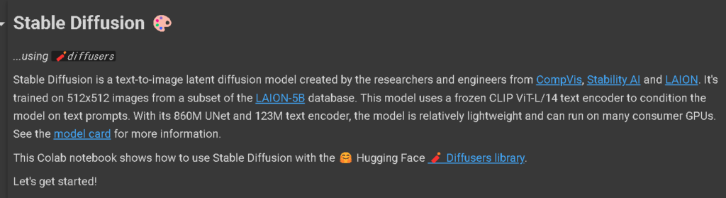
この英文ですね。
Stable Diffusion 🎨
...using 🧨diffusers
Stable Diffusion is a text-to-image latent diffusion model created by the researchers and engineers from CompVis, Stability AI and LAION. It's trained on 512x512 images from a subset of the LAION-5B database. This model uses a frozen CLIP ViT-L/14 text encoder to condition the model on text prompts. With its 860M UNet and 123M text encoder, the model is relatively lightweight and can run on many consumer GPUs. See the model card for more information.
This Colab notebook shows how to use Stable Diffusion with the 🤗 Hugging Face 🧨 Diffusers library.
Let's get started!
これの説明文をコピーしてDeepLで訳します。
👇日本語訳👇
Stable Diffusion 🎨
...using 🧨diffusers
Stable Diffusionは、CompVis, Stability AI, LAIONの研究者や技術者によって作られたテキストから画像への潜伏拡散モデルです。LAION-5Bデータベースのサブセットから512x512枚の画像で学習されています。このモデルは、凍結されたCLIP ViT-L/14テキストエンコーダを使用し、テキストプロンプトでモデルを条件付ける。860MのUNetと123Mのテキストエンコーダを持つこのモデルは、比較的軽量で、多くの民生用GPUで実行することができます。 詳しくはモデルカードをご覧ください。
このColabノートでは、🤗 Hugging Face 🧨Diffusers library を使って、Stable Diffusionを使用する方法を紹介します。
さっそく始めてみましょう
こんな感じです。
編集画面に貼り付け
ノートブックの該当部分に貼り付けるときは編集画面にする必要があります。
リンクしている文字を避けて、ブロック内をダブルクリック
すると、下の画像のような編集画面になります。
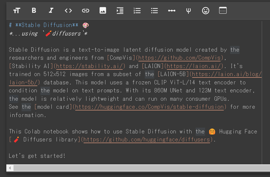
この状態で貼り付けることができます。
リンクに関しても、大体は大丈夫ですが、たまに「カッコ」が外れて、リンク以外のところもリンクに含まれたりしますが、カッコを見直して修正することができます。
ではこの調子で次も訳していきましょう。
How to use StableDiffusionPipeline
1. How to use StableDiffusionPipeline
Before diving into the theoretical aspects of how Stable Diffusion functions, let's try it out a bit 🤗.
In this section, we show how you can run text to image inference in just a few lines of code!
キーワードは訳さない方が良いし、How to useも訳すほどではないのでそのままです。
1. How to use StableDiffusionPipeline
Stable Diffusionがどのように機能するのか、理論的な側面に飛び込む前に、少し試してみましょう🤗。
このセクションでは、わずか数行のコードでテキストから画像への推論を実行できる方法を紹介します
絵文字はコピペや翻訳しても、ちゃんと残っていますね🤗。
次です。
Setup
Setup
First, please make sure you are using a GPU runtime to run this notebook, so inference is much faster. If the following command fails, use the Runtime menu above and select Change runtime type.
👇日本語訳👇
Setup
まず、このノートブックを実行するためにGPUランタイムを使用していることを確認してください、推論がより速くなります。以下のコマンドで失敗した場合は、上のランタイム メニューをクリックし、[ランタイム タイプの変更] を選択します。
この説明にある通り、GPUランタイムの設定をする必要がありますが、用語集の「Colaboratory」の項目の「GPUランタイムの設定方法」で解説していますのでご参照ください。
コードの解説
ここからは、コードの解説がメインになっていきますが、英語も訳していきます。
!nvidia-smi👇コードの解説👇
- 「!nvidia-smi」
- NVIDIA GPUの使用状況をモニタリングするコマンド
- このコマンドを実行すると
- GPUの種類
- 温度
- メモリ使用量
- プロセスID
- などの情報が表示される
- ノートブックを実行する前に
- GPUの状態を確認するために使われている
- !をつけると
- ノートブックのセルからシェルコマンドを実行できる
コードを実行するとコードの下にGPUの情報が表示されます。
Next, you should install diffusers as well scipy, ftfy and transformers. accelerate is used to achieve much faster loading.
👇日本語訳👇
次に、diffusersの他に、scipy、ftfy、transformersをインストールする必要があります。accelerate`は、より高速なロードを実現するために使用されます。
この説明通り、必要な diffusers、scipy、ftfy、transformers、accelerate をインストールする下記のコードがあるので実行しましょう。
!pip install diffusers==0.11.1
!pip install transformers scipy ftfy accelerateこれで、diffusers、scipy、ftfy、transformers、accelerate がインストールされました。
これ以降のコードでこれらの文字の下に波線が表示されていたら、このコードを再実行しましょう。
Stable Diffusion Pipeline
Stable Diffusion Pipeline
StableDiffusionPipeline is an end-to-end inference pipeline that you can use to generate images from text with just a few lines of code.
First, we load the pre-trained weights of all components of the model. In this notebook we use Stable Diffusion version 1.4 (CompVis/stable-diffusion-v1-4), but there are other variants that you may want to try:
- runwayml/stable-diffusion-v1-5
- stabilityai/stable-diffusion-2-1-base
- stabilityai/stable-diffusion-2-1. This version can produce images with a resolution of 768x768, while the others work at 512x512.
In addition to the model id CompVis/stable-diffusion-v1-4, we're also passing a specific revision and torch_dtype to the from_pretrained method.
We want to ensure that every free Google Colab can run Stable Diffusion, hence we're loading the weights from the half-precision branch fp16 and also tell diffusers to expect the weights in float16 precision by passing torch_dtype=torch.float16.
If you want to ensure the highest possible precision, please make sure to remove torch_dtype=torch.float16 at the cost of a higher memory usage.
👇日本語訳👇
Stable Diffusion Pipeline
StableDiffusionPipeline`はエンドツーエンドの推論パイプラインであり、数行のコードでテキストから画像を生成するために使用することができます。
まず、モデルのすべてのコンポーネントの事前学習された重みをロードします。このノートでは、Stable Diffusionのバージョン1.4を使っています。 (CompVis/stable-diffusion-v1-4), 他にもバリエーションがあるので、試してみてはいかがでしょうか。
- runwayml/stable-diffusion-v1-5
- stabilityai/stable-diffusion-2-1-base
- stabilityai/stable-diffusion-2-1 このバージョンは 768x768 の解像度で画像を生成できますが、他のバージョンは 512x512 で動作します。
モデル ID CompVis/stable-diffusion-v1-4 に加えて、特定のリビジョンと torch_dtype to も from_pretrained メソッドに渡します。
すべてのフリーのGoogle ColabがStable Diffusionを実行できるようにしたいので、半精度ブランチからウェイトをロードしています。 fp16 を使用し、 torch_dtype=torch.float16 を渡すことで、float16 精度の重みを期待するようにディフューザーに伝えます。
可能な限り高い精度を確保したい場合は、メモリ使用量が増えることを覚悟の上で、torch_dtype=torch.float16を必ず削除してください。
import torch~ コードの解説
いよいよPyTorchなど、機械学習のライブラリを準備していく段階に来ました。
import torch
from diffusers import StableDiffusionPipeline

pipe = StableDiffusionPipeline.from_pretrained("CompVis/stable-diffusion-v1-4", torch_dtype=torch.float16)
import torch ~
👇コードの解説👇
- import torch
- PythonでPyTorchという機械学習ライブラリを使うために必要なコード。
- PyTorch
- GPUを使って高速にテンソル計算や深層ニューラルネットワークを実行できるライブラリ
- import torch がエラーになる場合
- PyTorchのインストールが正しく行われていない可能性がある
StableDiffusionPipeline とは?
- StableDiffusionPipeline
- Stable Diffusionというテキストから画像を生成するモデルの一部
- Stable Diffusion
- CompVis, Stability AI, LAIONという企業や研究機関が開発したモデル
- LAION-5Bというデータセットの一部を使って512x512の画像を生成できる
- StableDiffusionPipelineクラス
- 画像生成のための処理をまとめたもの
- 関数のように呼び出す
- ノイズから画像が生成される過程を確認できる
では次に以下の部分のコードを解説します。
pipe = StableDiffusionPipeline.from_pretrained("CompVis/stable-diffusion-v1-4", torch_dtype=torch.float16)👇コードの解説👇
- StableDiffusionPipelineクラスのfrom_pretrainedメソッドを使用
- CompVis/stable-diffusion-v1-4モデルをダウンロード
- pipeという変数に代入
- CompVis/stable-diffusion-v1-4モデルをダウンロード
- 引数:torch_dtype=torch.float16を指定
- モデルのデータ型を16ビットの浮動小数点数にする
- メモリの使用量を減らすために行われる
Next, let's move the pipeline ~
Next, let's move the pipeline to GPU to have faster inference.
👇日本語訳👇
次に、パイプラインをGPUに移して、インターフェイスを高速化しましょう。
この文章に続いて下記のコードがあります。
pipe = pipe.to("cuda")👇コードの解説👇
- pipe(オブジェクト)をCUDA(デバイス)に移動させるもの
- CUDAとは
- NVIDIAのGPUを利用して高速な計算を行うための技術
- pipe.to(“cuda”)
- pipeの計算をGPUで行う
- CUDAとは
いよいよ画像生成!
And we are ready to generate images:
👇日本語訳👇
そして、画像を生成するための準備が整いました。
はい! 画像生成の準備が整いましたので、いよいよ画像生成ですね。
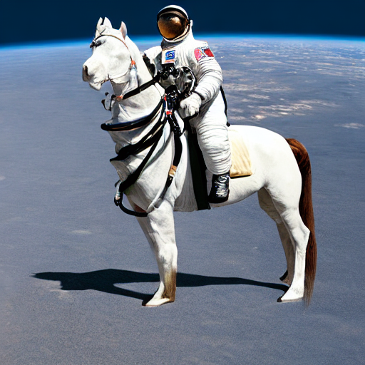
画像生成コード1:プロンプトを与える
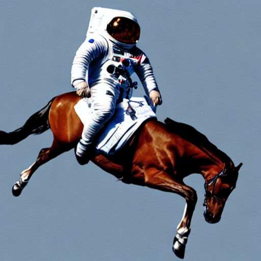
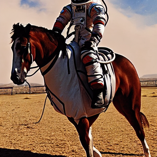
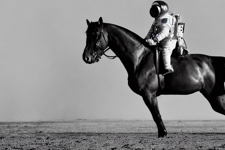
prompt = "a photograph of an astronaut riding a horse"
image = pipe(prompt).images[0]  # image here is in [PIL format](https://pillow.readthedocs.io/en/stable/)

# Now to display an image you can either save it such as:
image.save(f"astronaut_rides_horse.png")

# or if you're in a google colab you can directly display it with
image
👇コードの解説👇
- pipe(前出)にprompt(文字列)を渡して、画像を生成
- imageはpipeの返り値の中のimagesという属性の最初の要素
- PIL(画像処理ライブラリのフォーマット)で表される
画像を表示するには、image.saveというメソッドでファイルに保存するか、Google Colabなどのノートブック環境で直接imageを出力するかのどちらかです。
出力結果です。
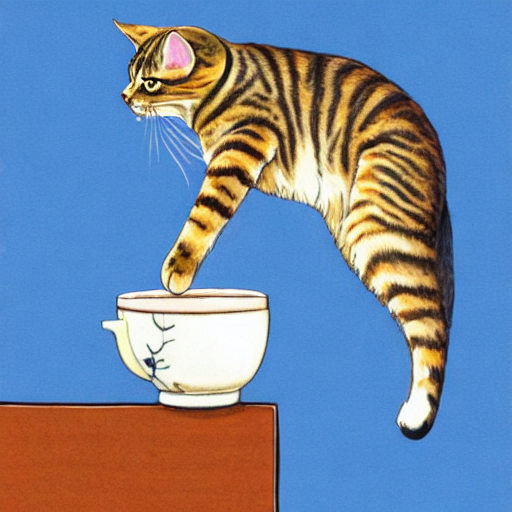
元のプロンプトをコメントアウトして、別のプロンプトを渡してみましょう。
# prompt = "a photograph of an astronaut riding a horse"
prompt = "a light brown tabby cat,tea time ,flying in the blue sky,manga"
出力結果です。
プロンプトの文章をいろいろ書き換えて画像生成を楽しんでください。
プロンプトの書き方のノウハウに関しては、たくさんの情報がありますので、そちらに譲ります。
ではもう少し、先に進んでいきましょう。
画像の下の説明文を訳します。
Running the above cell multiple times will give you a different image every time. If you want deterministic output you can pass a random seed to the pipeline. Every time you use the same seed you'll have the same image result.
👇日本語訳👇
上記のセルを複数回実行すると、毎回異なる画像を得ることができます。決定論的な出力が欲しい場合は、パイプラインにランダム シードを渡すことができます。同じ種を使うたびに、同じ画像の結果が得られます。
画像生成コード2:シード値を与える
今度は、シード値を与えて画像生成させるコードです。
import torch

generator = torch.Generator("cuda").manual_seed(1024)

image = pipe(prompt, generator=generator).images[0]

image
👇コードの解説👇
- PyTorchを使い
- stable-diffusionのモデルを呼び出し
- テキストのプロンプトから画像を生成する
- stable-diffusionのモデルを呼び出し
- PyTorchをインポート
- PyTorch:テンソル(多次元配列)を使い
- 機械学習の計算を行うことができるライブラリ
- PyTorch:テンソル(多次元配列)を使い
- generator = torch.Generator(“cuda”).manual_seed(1024)
- ランダムな数を生成するためのオブジェクトを作る
- generatorという変数に代入
- torch.Generator関数
- PyTorchのランダム数生成器を作るためのもの
- "cuda":GPUを指定
- manual_seedメソッド
- ランダム数生成器のシード値を設定するためのもの
- シード値
- ランダムな数の生成に影響する値
- 同じシード値を使うと、同じランダムな数を生成
- 1024:シード値として選んだ任意の数
- ランダムな数を生成するためのオブジェクトを作る
- image = pipe(prompt, generator=generator).images[0]
- stable-diffusionのモデルでプロンプトから画像を生成
- pipeオブジェクトに、promptとgeneratorを引数として渡す
- generator:先ほど作ったランダム数生成器
- pipe
- プロンプトとランダム数生成器を受け取る
- 画像を生成
- 生成された画像
- pipeオブジェクトのimages属性に格納される
- images属性は、複数の画像を要素とするリスト
- リストの0番目の要素を取り出す
- [0]というインデックスを使う
- 取り出された画像:imageという変数に代入される
- プロンプトとランダム数生成器を受け取る
- stable-diffusionのモデルでプロンプトから画像を生成
- 生成された画像を表示
- imageという変数に代入された画像
- PyTorchのテンソルという形式
- 「image」を実行すると、画像として表示される
- imageという変数に代入された画像
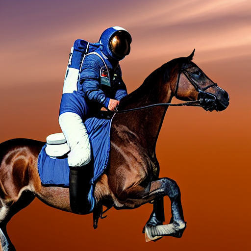
出力結果です。
manual_seed(1024) の数字をいろいろ変えて画像を出力すると、同じプロンプトでも、かなり違った雰囲気の画像が生成されますので、試してみましょう。
上の画像は manual_seed の数字を128、256、512 に変えて実行した結果です(8の倍数以外でもOKです)。
画像生成コード3:推論ステップ数の変更
次は、推論ステップ数を変更するサンプルコードです。
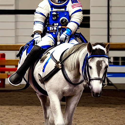
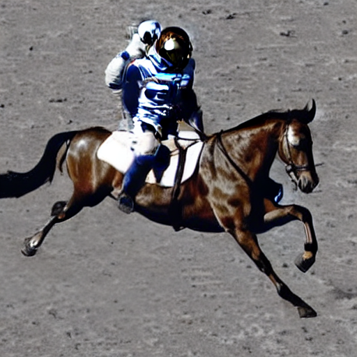
You can change the number of inference steps using the num_inference_steps argument. In general, results are better the more steps you use. Stable Diffusion, being one of the latest models, works great with a relatively small number of steps, so we recommend to use the default of 50. If you want faster results you can use a smaller number.
The following cell uses the same seed as before, but with fewer steps. Note how some details, such as the horse's head or the helmet, are less defin realistic and less defined than in the previous image:
👇日本語訳👇
引数 num_inference_steps を使って推論ステップ数を変更することができます。一般的に、結果はより多くのステップを使用するほど良くなります。Stable Diffusionは最新のモデルの1つであり、比較的少ないステップ数でうまく機能するため、デフォルトの50を使用することをお勧めします。もし、より速い結果を得たいのであれば、より小さな数を使用することができます。
次のセルは、前と同じシードを使用していますが、より少ないステップ数です。馬の頭やヘルメットのような細部は、前の画像に比べて、リアルでなく、明確に表現されていないことに注意してください。
「num_inference_steps は、デフォルトの50がおすすめだけど、いろいろ試してみて」ということでしょうね。
出力結果です。
画像の下の説明文を訳します。
The other parameter in the pipeline call is guidance_scale. It is a way to increase the adherence to the conditional signal which in this case is text as well as overall sample quality. In simple terms classifier free guidance forces the generation to better match with the prompt. Numbers like 7 or 8.5 give good results, if you use a very large number the images might look good, but will be less diverse.
👇日本語訳👇
パイプラインコールのもう一つのパラメータは guidance_scale です。これは、条件付き信号(この場合はテキスト)および全体的なサンプルの品質への準拠を高めるための方法です。簡単に言うと、分類子を使わないガイダンスは、よりプロンプトにマッチするように生成を強制します。「7」や「8.5」のような数字は良い結果をもたらしますが、非常に大きな数字を使用した場合、画像は良く見えるかもしれませんが、多様性に欠けることになります。
guidance_scale というキーワードが出てきますが、実際にコードの中で出てくるのは、かなり後の方です。
「パイプラインコールには、もう一つパラメータがあるよ」とここで言っておきたかったのでしょう。
画像生成コード4:複数画像生成(1行×3列)
まず説明文を訳していきます。
To generate multiple images for the same prompt, we simply use a list with the same prompt repeated several times. We'll send the list to the pipeline instead of the string we used before.
👇日本語訳👇
同じプロンプトに対して複数の画像を生成するには、同じプロンプトを複数回繰り返したリストを使用するだけです。先ほど使った文字列の代わりに、このリストをパイプラインに送ります。
つまり、箇条書きにすると以下のようになります。
- 同じプロンプトに対して複数の画像を生成するには
- 同じプロンプトを複数回繰り返したリストを使用
- リストをパイプラインに送る
- 同じプロンプトを複数回繰り返したリストを使用
説明文を訳します。
Let's first write a helper function to display a grid of images. Just run the following cell to create the image_grid function, or disclose the code if you are interested in how it's done.
👇日本語訳👇
まず、画像のグリッドを表示するためのヘルパー関数を書いてみましょう。以下のセルを実行するだけでimage_grid関数が作成されます。どのように行われているのか興味がある方はコードを開示してください。
処理を使い回し、作業効率を上げるためのヘルパー関数を用意するということですね。
次のコードが、そのヘルパー関数です。
from PIL import Image

def image_grid(imgs, rows, cols):
    assert len(imgs) == rows*cols

    w, h = imgs[0].size
    grid = Image.new('RGB', size=(cols*w, rows*h))
    grid_w, grid_h = grid.size

    for i, img in enumerate(imgs):
        grid.paste(img, box=(i%cols*w, i//cols*h))
    return grid
👇コードの解説👇
- image_grid 関数
- 引数:imgs, rows, cols(画像リスト、行数、列数)
- imgsの長さがrows*colsと等しいことを確認
- そうでない場合は、エラーを発生させる
- imgsの最初の画像のサイズをwとhという変数に代入
- gridという新しい画像を作成
- 画像のサイズ:cols*wとrows*hとする
- imgsの画像をrows行cols列に並べたときのサイズ
- 画像のサイズ:cols*wとrows*hとする
- gridのサイズをgrid_wとgrid_hという変数に代入
- imgsの画像を順番に取り出し、gridに貼り付ける
- 貼り付ける位置:インデックス「i」に応じて計算
- 「i」は0始まり
- i%cols*w:列の位置を表す
- i//cols*h:行の位置を表す
- gridを返す
コードを実行して、下記の説明文を読みましょう。
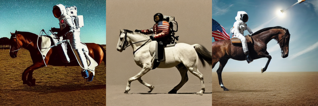
Now, we can generate a grid image once having run the pipeline with a list of 3 prompts.
👇日本語訳👇
これで、3つのプロンプトのリストでパイプラインを実行すれば、グリッド画像を生成することができるようになりました。
グリッド画像を生成する準備が整いましたので、次のコードを実行しましょう。
num_images = 3
prompt = ["a light brown tabby cat,tea time ,flying in the blue sky,manga"] * num_images

images = pipe(prompt).images

grid = image_grid(images, rows=1, cols=3)
grid
👇コードの解説👇
- num_images変数
- 「3」を代入
- 生成する画像の数
- 「3」を代入
- prompt変数
- [“プロンプトの文”]のリストをnum_images倍して代入
- 画像の生成に使うテキストのリスト
- リストの要素は、カンマで区切られた複数のテキスト
- リストの長さは、num_imagesと同じ
- [“プロンプトの文”]のリストをnum_images倍して代入
- imagesという変数に、pipe(prompt).imagesという式の結果を代入します。これは、promptのテキストを使って画像を生成する関数です。pipeという関数は、OpenAIのDALL-Eというモデルを使っています。imagesは、生成された画像のリストです。
- gridという変数に、image_grid(images, rows=1, cols=3)という関数の結果を代入します。これは、前に定義したヘルパー関数です。imagesの画像を1行3列に並べた画像を作ります。
- gridを表示します。これは、生成された画像のグリッドです。
出力結果です。
画像生成コード5:複数画像生成(4行×3列)
今度は、n × mでグリッドの数を変更できるコードのサンプルです。
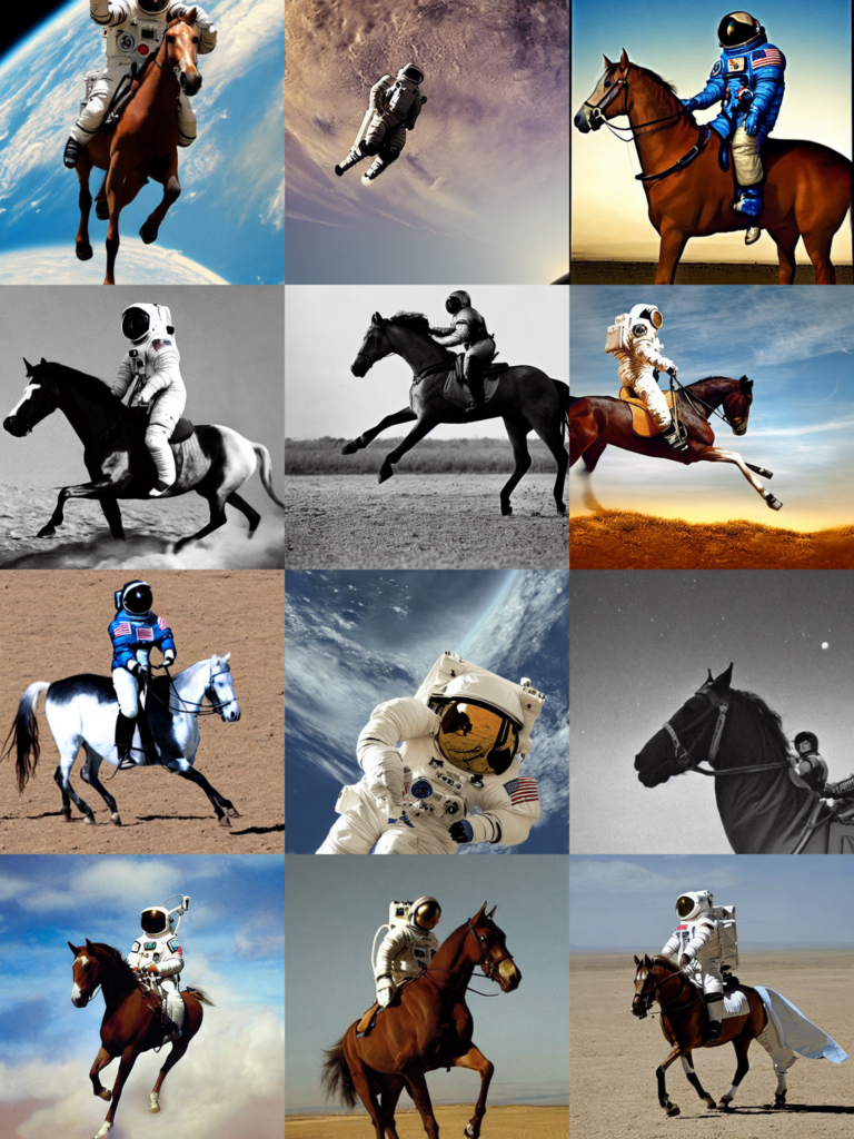
And here's how to generate a grid of n × m images.
👇日本語訳👇
n × m 画像のグリッドを生成する方法は次のとおりです。
ではコードを見てみましょう。
num_cols = 3
num_rows = 4

prompt = ["a photograph of an astronaut riding a horse"] * num_cols

all_images = []
for i in range(num_rows):
  images = pipe(prompt).images
  all_images.extend(images)

grid = image_grid(all_images, rows=num_rows, cols=num_cols)
grid
👇コードの解説👇
- num_cols、num_rows
- 生成する画像の列数、行数
- prompt変数
- [プロンプト文]をnum_cols倍して代入
- 画像の生成用リスト
- リストの長さは、num_colsと同じになる
- [プロンプト文]をnum_cols倍して代入
- all_images
- 生成された画像を保存するリスト
- for文
- 「i」を0からnum_rows-1まで変化させる
- 行の数だけ繰り返すループ
- 「i」を0からnum_rows-1まで変化させる
- images
- pipe(prompt).imagesという式の結果を代入
- promptのテキストを使って画像を生成する関数
- pipe(prompt).imagesという式の結果を代入
- all_images
- extendメソッドを使用してimagesを追加
- extend:リストに別のリストの要素をすべて追加するメソッド
- extendメソッドを使用してimagesを追加
- for文終了後
- gridにimage_grid関数の結果を代入
- 前に定義したヘルパー関数
- gridにimage_grid関数の結果を代入
- grid
- 生成された画像のグリッドを表示
出力結果です。
画像生成コード6:縦長、横長画像の生成
今までは正方形だけでしたが、今度は縦長や横長画像の生成のサンプルコードです。
Generate non-square images
Stable Diffusion produces images of 512 × 512 pixels by default. But it's very easy to override the default using the height and width arguments, so you can create rectangular images in portrait or landscape ratios.
These are some recommendations to choose good image sizes:
- Make sure
heightandwidthare both multiples of8. - Going below 512 might result in lower quality images.
- Going over 512 in both directions will repeat image areas (global coherence is lost).
- The best way to create non-square images is to use
512in one dimension, and a value larger than that in the other one.
👇日本語訳👇
非正方形の画像を生成する
Stable Diffusionは、デフォルトで512×512ピクセルの画像を作成します。しかし、heightとwidthの引数を使ってデフォルトを上書きするのはとても簡単なので、縦長や横長の長方形の画像を作成することができます。
以下は、適切な画像サイズを選択するためのいくつかの推奨事項です。
高さと幅がともに8の倍数であることを確認してください。
512を下回ると、低品質の画像になる可能性があります。
縦横ともに512を超えると、画像領域が繰り返されます(全体的なまとまりが失われます)。
正方形でない画像を作成するには、1つの次元に512を使用し、もう1つの次元にそれよりも大きな値を使用するのが最も良い方法です。
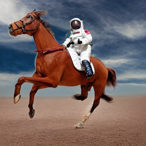
prompt = "a photograph of an astronaut riding a horse"

image = pipe(prompt, height=512, width=768).images[0]
image
👇コードの解説👇
- pipe
- 引数の height, widthに横長になる値を渡している
- 条件:8の倍数
- 引数の height, widthに横長になる値を渡している
出力結果です。
What is Stable Diffusion
このあたりから「Stable Diffusion」の理論的な長い説明になるので、対訳が続きます。
What is Stable Diffusion
Now, let's go into the theoretical part of Stable Diffusion 👩🎓.
Stable Diffusion is based on a particular type of diffusion model called Latent Diffusion, proposed in High-Resolution Image Synthesis with Latent Diffusion Models.
👇日本語訳👇
Stable Diffusion(安定拡散)とは
さて、Stable Diffusion 👩🎓 の理論的な部分について説明します。
Stable Diffusionは、High-Resolution Image Synthesis with Latent Diffusion Modelsで提案されたLatent Diffusionという特殊な拡散モデルに基づいています。
一般的な拡散モデルとの対比
続けて次のブロックを訳します。
General diffusion models are machine learning systems that are trained to denoise random gaussian noise step by step, to get to a sample of interest, such as an image. For a more detailed overview of how they work, check this colab.
Diffusion models have shown to achieve state-of-the-art results for generating image data. But one downside of diffusion models is that the reverse denoising process is slow. In addition, these models consume a lot of memory because they operate in pixel space, which becomes unreasonably expensive when generating high-resolution images. Therefore, it is challenging to train these models and also use them for inference.
👇日本語訳👇
一般的な拡散モデルは、ランダムなガウスノイズを段階的にノイズ除去するように訓練された機械学習システムで、画像などの目的のサンプルに到達するために使用されます。より詳細な仕組みについては、こちらのcolabをご覧ください。
拡散モデルは、画像データの生成において、最先端の結果を達成することが示されています。しかし、拡散モデルの欠点は、逆ノイズ処理に時間がかかることです。また、これらのモデルはピクセル空間で動作するため、多くのメモリを消費し、高解像度の画像を生成する場合には不当に高価になります。そのため、これらのモデルを訓練し、さらに推論に使用することは困難です。
続けて次のブロックを訳します。
Latent diffusion can reduce the memory and compute complexity by applying the diffusion process over a lower dimensional latent space, instead of using the actual pixel space. This is the key difference between standard diffusion and latent diffusion models: in latent diffusion the model is trained to generate latent (compressed) representations of the images.
There are three main components in latent diffusion.
- An autoencoder (VAE).
- A U-Net.
- A text-encoder, e.g. CLIP's Text Encoder.
👇日本語訳👇
潜在拡散は、実際のピクセル空間を使用する代わりに、低次元の潜在空間上で拡散プロセスを適用することにより、メモリと計算の複雑さを軽減することができます。これが標準的な拡散と潜伏拡散モデルの主な違いです。潜伏拡散では、モデルは画像の潜伏(圧縮)表現を生成するように訓練されます。
潜像拡散には3つの主要なコンポーネントがあります。
- オートエンコーダ(VAE)
- U-Net(ユーネット)
- テキストエンコーダ(CLIPのテキストエンコーダなど)
1.オートエンコーダ(VAE)について
続けて次のブロックを訳します。
1. The autoencoder (VAE)
The VAE model has two parts, an encoder and a decoder. The encoder is used to convert the image into a low dimensional latent representation, which will serve as the input to the U-Net model. The decoder, conversely, transforms the latent representation back into an image.
During latent diffusion training, the encoder is used to get the latent representations (latents) of the images for the forward diffusion process, which applies more and more noise at each step. During inference, the denoised latents generated by the reverse diffusion process are converted back into images using the VAE decoder. As we will see during inference we only need the VAE decoder.
👇日本語訳👇
- オートエンコーダ(VAE)
VAEモデルには、エンコーダーとデコーダーの2つの部分があります。エンコーダーは、画像を低次元の潜在表現に変換し、U-Netモデルの入力として使用します。デコーダは、逆に潜在表現を画像に変換する。
潜像拡散学習では、エンコーダは、各ステップでより多くのノイズを適用する順拡散プロセスのために、画像の潜像表現(レイテント)を得るために使用されます。推論では、逆拡散処理で生成された潜在能力を、VAEデコーダで画像に戻します。後述するように、推論時に必要なのはVAEデコーダだけである。
2.The U-Netについて
続けて次のブロックを訳します。
2. The U-Net
The U-Net has an encoder part and a decoder part both comprised of ResNet blocks. The encoder compresses an image representation into a lower resolution image representation and the decoder decodes the lower resolution image representation back to the original higher resolution image representation that is supposedly less noisy. More specifically, the U-Net output predicts the noise residual which can be used to compute the predicted denoised image representation.
To prevent the U-Net from losing important information while downsampling, short-cut connections are usually added between the downsampling ResNets of the encoder to the upsampling ResNets of the decoder. Additionally, the stable diffusion U-Net is able to condition its output on text-embeddings via cross-attention layers. The cross-attention layers are added to both the encoder and decoder part of the U-Net usually between ResNet blocks.
👇日本語訳👇
- U-NETについて
U-Netは、ResNetブロックで構成されたエンコーダ部とデコーダ部を備えています。エンコーダは画像表現を低解像度画像表現に圧縮し、デコーダは低解像度画像表現を、ノイズが少ないとされる元の高解像度画像表現に復号する。より具体的には、U-Netの出力は、予測されたノイズ除去された画像表現を計算するために使用できるノイズ残差を予測します。
U-Netがダウンサンプリング中に重要な情報を失うのを防ぐため、通常、エンコーダのダウンサンプリングResNetsとデコーダのアップサンプリングResNetsの間にショートカットの接続が追加される。さらに、安定拡散U-Netは、クロスアテンションレイヤーを介して、テキストエンベッディングに出力を条件付けることができる。クロスアテンションレイヤーは、U-Netのエンコーダ部とデコーダ部の両方に、通常ResNetブロックの間に追加されます。
3.テキストエンコーダについて
続けて次のブロックを訳します。
3. The Text-encoder
The text-encoder is responsible for transforming the input prompt, e.g. "An astronout riding a horse" into an embedding space that can be understood by the U-Net. It is usually a simple transformer-based encoder that maps a sequence of input tokens to a sequence of latent text-embeddings.
Inspired by Imagen, Stable Diffusion does not train the text-encoder during training and simply uses an CLIP's already trained text encoder, CLIPTextModel.
👇日本語訳👇
- テキストエンコーダ
テキストエンコーダは、入力されたプロンプト、例えば "An astronout riding a horse "を、U-Netが理解できる埋め込み空間に変換する役割を担っています。これは通常、入力トークンのシーケンスを潜在的なテキスト埋込みのシーケンスにマッピングする単純な変換器ベースのエンコーダである。
Imagenに触発されたStable Diffusionは、学習中にテキストエンコーダを訓練せず、単にCLIPの既に訓練されたテキストエンコーダ、CLIPTextModelを使用します。
なぜ潜伏拡散は高速で効率的なのか?
続けて次のブロックを訳します。
Why is latent diffusion fast and efficient?
Since the U-Net of latent diffusion models operates on a low dimensional space, it greatly reduces the memory and compute requirements compared to pixel-space diffusion models. For example, the autoencoder used in Stable Diffusion has a reduction factor of 8. This means that an image of shape (3, 512, 512) becomes (3, 64, 64) in latent space, which requires 8 × 8 = 64 times less memory.
This is why it's possible to generate 512 × 512 images so quickly, even on 16GB Colab GPUs!
👇日本語訳👇
なぜ潜伏拡散は高速で効率的なのか?
潜在拡散モデルのU-Netは低次元空間で動作するため、ピクセル空間の拡散モデルと比較してメモリや計算量を大幅に削減することができます。例えば、Stable Diffusionで使用されるオートエンコーダは、縮小率が8であり、これは、形状が(3, 512, 512)の画像が潜像空間では(3, 64, 64)となり、8×8=64倍のメモリを必要とすることを意味しています。
これが、16GBのColab GPUでも、512×512の画像を高速に生成できる理由です
推論中の安定した拡散
続けて次のブロックを訳します。
Stable Diffusion during inference
Putting it all together, let's now take a closer look at how the model works in inference by illustrating the logical flow.
👇日本語訳👇
推論中の安定した拡散
このように、論理的な流れを示すことで、推論においてモデルがどのように機能するのかを詳しく見ていきましょう。
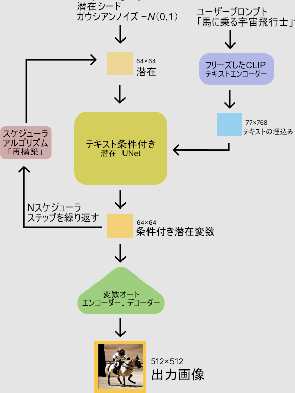
以下の図も頑張って日本語のラベルを貼ってみました。
続けて次のブロックを訳します。
The stable diffusion model takes both a latent seed and a text prompt as an input. The latent seed is then used to generate random latent image representations of size 64×64 where as the text prompt is transformed to text embeddings of size 77×768 via CLIP's text encoder.
Next the U-Net iteratively denoises the random latent image representations while being conditioned on the text embeddings. The output of the U-Net, being the noise residual, is used to compute a denoised latent image representation via a scheduler algorithm. Many different scheduler algorithms can be used for this computation, each having its pros and cons. For Stable Diffusion, we recommend using one of:
- PNDM scheduler (used by default).
- K-LMS scheduler.
- Heun Discrete scheduler.
- DPM Solver Multistep scheduler. This scheduler is able to achieve great quality in less steps. You can try with 25 instead of the default 50!
Theory on how the scheduler algorithm function is out of scope for this notebook, but in short one should remember that they compute the predicted denoised image representation from the previous noise representation and the predicted noise residual. For more information, we recommend looking into Elucidating the Design Space of Diffusion-Based Generative Models
The denoising process is repeated ca. 50 times to step-by-step retrieve better latent image representations. Once complete, the latent image representation is decoded by the decoder part of the variational auto encoder.
After this brief introduction to Latent and Stable Diffusion, let's see how to make advanced use of 🤗 Hugging Face Diffusers!
👇日本語訳👇
stable diffusion(安定拡散)モデルは、潜在的な種とテキストプロンプトの両方を入力として受け取る。潜伏種は64×64サイズのランダムな潜像表現を生成するために用いられ、テキストプロンプトはCLIPのテキストエンコーダによって77×768サイズのテキスト埋め込みに変換される。
次にU-Netは、テキスト埋め込みを条件としながら、ランダムな潜像表現を繰り返しノイズ除去する。U-Netの出力はノイズ残差であり、スケジューラアルゴリズムによってノイズ除去された潜像表現を計算するために使用される。この計算には多くの異なるスケジューラアルゴリズムを使用することができ、それぞれに長所と短所がある。Stable Diffusionでは、以下のいずれかを使用することを推奨します。
PNDMスケジューラー(デフォルトで使用されています)。
K-LMSスケジューラー
Heun Discreteスケジューラー
DPM Solver Multistepスケジューラー。このスケジューラーは、より少ないステップで優れた品質を実現することができます。デフォルトの50ステップではなく、25ステップで試してみてください。
スケジューラアルゴリズムの機能に関する理論は、このノートブックの範囲外ですが、要するに、以前のノイズ表現と予測ノイズ残差から、予測ノイズ除去画像表現を計算することを覚えておくとよいでしょう。より詳細な情報については、「拡散に基づく生成モデルのデザイン空間を解明する」を参照されたい。
このノイズ除去処理を約50回繰り返すことで、より良い潜像表現を段階的に取得する。潜像表現は、変分オートエンコーダのデコーダ部によって復号化される。
このように、「潜熱拡散」と「安定拡散」を簡単に紹介した後は、「🤗ハギングフェイスディフューザー」の高度な活用法を見ていきましょう!
続けて次のブロックを訳します。
ディフューザーを使った独自の推論パイプラインの書き方
How to write your own inference pipeline with diffusers
Finally, we show how you can create custom diffusion pipelines with diffusers. This is often very useful to dig a bit deeper into certain functionalities of the system and to potentially switch out certain components.
In this section, we will demonstrate how to use Stable Diffusion with a different scheduler, namely Katherine Crowson's K-LMS scheduler that was added in this PR.
👇日本語訳👇
ディフューザーを使った独自の推論パイプラインの書き方
最後に、ディフューザーを使ってカスタムディフュージョンパイプラインを作成する方法について紹介します。これは、システムの特定の機能をもう少し深く掘り下げたり、特定のコンポーネントを入れ替える可能性がある場合に、しばしば非常に便利です。
このセクションでは、異なるスケジューラー、すなわち今回のPRで追加されたKatherine CrowsonのK-LMSスケジューラーでStable Diffusionを使用する方法を示します。
続けて次のブロックを訳します。
Let's go through the StableDiffusionPipeline step by step to see how we could have written it ourselves.
We will start by loading the individual models involved.
👇日本語訳👇
それでは、StableDiffusionPipelineを自分たちでどのように書いたか、順を追って見ていきましょう。
まず、関係する個々のモデルをロードすることから始めます。
CUDAというGPUを使うための技術が利用可能かどうかを返す関数
やっと久しぶりにコードが出てきました。
import torch
torch_device = "cuda" if torch.cuda.is_available() else "cpu"
👇コードの解説👇
- torch_device変数
- if~else文
- "cuda"か"cpu"どちらかを代入
- 条件:torch.cuda.is_available()という関数の結果
- if~else文
- torch.cuda.is_available()
- CUDAというGPUを使うための技術が利用可能かどうかを返す関数
- CUDAという技術が
- 利用可能:"cuda"を代入
- 利用不可能:"cpu"を代入
- torch_deviceという変数は、PyTorchのテンソルやモデルをどのデバイスで計算するかを指定するために使われる
- CUDAという技術が
- CUDAというGPUを使うための技術が利用可能かどうかを返す関数
続けて次のブロックを訳します。
The pre-trained model includes all the components required to setup a complete diffusion pipeline. They are stored in the following folders:
text_encoder: Stable Diffusion uses CLIP, but other diffusion models may use other encoders such asBERT.tokenizer. It must match the one used by thetext_encodermodel.scheduler: The scheduling algorithm used to progressively add noise to the image during training.unet: The model used to generate the latent representation of the input.vae: Autoencoder module that we'll use to decode latent representations into real images.
We can load the components by referring to the folder they were saved, using the subfolder argument to from_pretrained.
👇日本語訳👇
訓練済みモデルには、完全な拡散パイプラインをセットアップするために必要なすべてのコンポーネントが含まれています。これらは、以下のフォルダに格納されています。
- text_encoder
- Stable DiffusionはCLIPを使用していますが、他の拡散モデルではBERTなど他のエンコーダを使用することがあります。
- トークナイザー:text_encoderモデルで使用されているものと一致する必要があります。
- スケジューラ:トレーニング中に画像にノイズを徐々に追加するために使用されるスケジューリングアルゴリズム。
- unet:入力の潜在的な表現を生成するために使用されるモデル。
- vae: 潜在表現を実画像にデコードするために使用するオートエンコーダーモジュール。
from_pretrainedのサブフォルダ引数を用いて、保存されたフォルダを参照することで、コンポーネントをロードすることができます。
CLIPと潜在拡散モデルを用いた画像生成の準備
ここで、コードの解説です。
from transformers import CLIPTextModel, CLIPTokenizer
from diffusers import AutoencoderKL, UNet2DConditionModel, PNDMScheduler

# 1. Load the autoencoder model which will be used to decode the latents into image space.
vae = AutoencoderKL.from_pretrained("CompVis/stable-diffusion-v1-4", subfolder="vae")

# 2. Load the tokenizer and text encoder to tokenize and encode the text.
tokenizer = CLIPTokenizer.from_pretrained("openai/clip-vit-large-patch14")
text_encoder = CLIPTextModel.from_pretrained("openai/clip-vit-large-patch14")

# 3. The UNet model for generating the latents.
unet = UNet2DConditionModel.from_pretrained("CompVis/stable-diffusion-v1-4", subfolder="unet")
👇コードの解説👇
- transformersモジュールから以下のクラスを読み込む
- CLIPTextModelクラス
- CLIPTokenizerクラス
- diffusersモジュールから以下のクラスを読み込む
- AutoencoderKLクラス
- UNet2DConditionModelクラス
- PNDMSchedulerクラス
- transformersモジュール
- Hugging Face(会社)が提供
- 自然言語処理のための
- モデルやトークナイザーを使うためのモジュール
- 自然言語処理のための
- Hugging Face(会社)が提供
- CLIPTextModelクラス、CLIPTokenizerクラス
- OpenAIのCLIPというモデルを使うためのクラス
- CLIPモデルは、テキストと画像の間の関連性を学習するモデル
- diffusersモジュール
- CompVisチームが提供する画像生成のためのモデルやスケジューラーを使うためのモジュール
- AutoencoderKL、UNet2DConditionModel、PNDMSchedulerクラス
- 安定した拡散という手法を使うためのクラス
- 安定した拡散という手法
- 画像をノイズに変える逆過程を学習
- 画像を生成する手法
- 画像をノイズに変える逆過程を学習
- vae変数
- AutoencoderKLクラスのfrom_pretrainedメソッドの結果を代入
- from_pretrainedメソッド
- 事前に学習されたモデルを読み込む
- 引数:
- "CompVis/stable-diffusion-v1-4"
- subfolderに"vae"を渡す
- CompVisというチームが提供する安定した拡散のモデルのうち、サブフォルダ「vae」にあるモデルを読み込む
- vae変数:オートエンコーダというモデル
- 画像を低次元の潜在変数に圧縮
- 潜在変数から画像に復元
- tokenizer変数
- CLIPTokenizerクラスのfrom_pretrainedメソッドの結果を代入
- from_pretrainedメソッド
- 事前に学習されたトークナイザーを読み込む
- 引数:"openai/clip-vit-large-patch14"
- OpenAIのCLIPモデルのVision Transformerモデルを使った大きなサイズのモデルのトークナイザーを読み込む
- tokenizer変数は、トークナイザーというモデル
- トークナイザーモデル
- テキストを
- 単語や文字のような小さな単位に分割
- 数値に変換
- テキストを
K-LMSのスケジューラー
続けて次のブロックを訳します。
Now instead of loading the pre-defined scheduler, we'll use the K-LMS scheduler instead.
👇日本語訳👇
今度は、あらかじめ用意されたスケジューラーを読み込むのではなく、K-LMSのスケジューラーを使うことにします。
ここでコードとその解説です。
from diffusers import LMSDiscreteScheduler

scheduler = LMSDiscreteScheduler.from_pretrained("CompVis/stable-diffusion-v1-4", subfolder="scheduler")
👇コードの解説👇
- diffusersモジュールから以下のクラスを読み込む
- LMSDiscreteSchedulerクラス
- diffusersモジュール
- 画像生成のためのモデルやschedulerを使うためのモジュール
- LMSDiscreteSchedulerクラス
- 安定した拡散のスケジューラーの一種
- schedulerモデル
- 安定した拡散の過程で使われるパラメーターを決めるモデル
- scheduler変数
- LMSDiscreteSchedulerクラスのfrom_pretrainedメソッドの結果を代入
- from_pretrainedメソッド
- 事前に学習されたスケジューラーを読み込むメソッド
- 引数:"CompVis/stable-diffusion-v1-4"
- subfolder(キーワード引数)に"scheduler"を渡す
- CompVisチーム提供の安定した拡散のモデルのうち、サブフォルダ「scheduler」にあるモデルを読み込む
- scheduler(変数)
- LMSDiscreteSchedulerモデル
- 安定した拡散のパラメーターを離散的に決める
- LMSDiscreteSchedulerモデル
モデルをGPUに移動
続けて次のブロックを訳します。
Next we move the models to the GPU.
👇日本語訳👇
次に、モデルをGPUに移動させます。
ここでコードとその解説です。
vae = vae.to(torch_device)
text_encoder = text_encoder.to(torch_device)
unet = unet.to(torch_device)
👇コードの解説👇
- vae変数に代入されたオートエンコーダモデル
- toメソッドを使い、torch_device変数に代入されたデバイスに移動
- toメソッド
- モデルやテンソルを別のデバイスに移動するメソッド
- デバイス:計算を行うためのハードウェアのこと
- 例えば、CPUやGPUなど
- torch_device変数
- torchモジュールのdeviceクラスのインスタンス
- torchモジュール
- PyTorch(深層学習のためのフレームワーク)を使うためのモジュール
- deviceクラス
- デバイスの種類や番号を表すクラス
- text_encoder変数に代入されたテキストエンコーダーモデル
- toメソッドを使い、torch_device変数に代入されたデバイスに移動
- unet変数に代入されたUNetモデル
- toメソッドを使い、torch_device変数に代入されたデバイスに移動
画像生成に使用するパラメータを定義
続けて次のブロックを訳します。
We now define the parameters we'll use to generate images.
Note that guidance_scale is defined analog to the guidance weight w of equation (2) in the Imagen paper. guidance_scale == 1 corresponds to doing no classifier-free guidance. Here we set it to 7.5 as also done previously.
In contrast to the previous examples, we set num_inference_steps to 100 to get an even more defined image.
👇日本語訳👇
ここで、画像生成に使用するパラメータを定義します。
guidance_scaleは、Imagen論文の式(2)のガイダンス重みwに類似して定義されていることに注意してください。guidance_scale == 1は、分類子を使わないガイダンスを行うことに相当します。ここでは、前回と同様に7.5に設定しています。
また、num_inference_stepsを100に設定することで、より明確なイメージを得ることができます。
ここでコードとその解説です。
prompt = ["a photograph of an astronaut riding a horse"]
height = 512 # default height of Stable Diffusion
width = 512 # default width of Stable Diffusion
num_inference_steps = 100 # Number of denoising steps
guidance_scale = 7.5 # Scale for classifier-free guidance
generator = torch.manual_seed(32) # Seed generator to create the inital latent noise
batch_size = 1
👇コードの解説👇
- prompt変数
- [プロンプト文]のリストを代入
- height変数、width変数に、512を代入
- 生成する画像の高さをピクセル単位で表したもの
- 512は、安定した拡散のモデルのデフォルトの高さ
- num_inference_steps変数
- 100を代入
- 画像生成のための脱ノイズのステップ数
- 脱ノイズとは、画像を徐々に鮮明にする過程
- 100は、脱ノイズのステップ数の推奨値
- 100を代入
- guidance_scale変数
- 7.5を代入
- 分類器を使わないガイダンスのスケールを表したもの
- 分類器を使わないガイダンス
- テキストエンコーダーとUNetモデルを使い
- テキスト入力に沿った画像を生成する方法
- スケールとは、ガイダンスの強さを表すパラメーター
- 7.5はガイダンスのスケールの推奨値
- テキストエンコーダーとUNetモデルを使い
- 7.5を代入
- generator変数
- torchモジュールのmanual_seed関数の結果を代入
- manual_seed関数
- 乱数生成器のシードを設定する
- シード
- 乱数生成器の初期値
- 引数:32(シード値)
- シードを渡す
- 乱数生成器の出力が固定される
- 乱数生成器
- 画像生成のための初期の潜在ノイズを作るのに使われる
- 乱数生成器の初期値
- batch_size変数
- 1を代入
- 画像生成のためのバッチサイズを表したもの
- バッチサイズ
- 一度に処理するデータの数
- 1はバッチサイズの最小値
- 1を代入
UNetモデルの条件付け
続けて次のブロックを訳します。
First, we get the text_embeddings for the prompt. These embeddings will be used to condition the UNet model.
👇日本語訳👇
まず、プロンプトのtext_embeddingsを取得する。これらのembeddings(埋め込み)はUNetモデルの条件付けに使われる。
ここでコードとその解説です。
text_input = tokenizer(prompt, padding="max_length", max_length=tokenizer.model_max_length, truncation=True, return_tensors="pt")
with torch.no_grad():
text_embeddings = text_encoder(text_input.input_ids.to(torch_device))[0]
👇コードの解説👇
このコードは、テキストをベクトルに変換するためのもの
- tokenizer関数
- prompt変数に入っているテキストを単語に分割
- padding, max_length, truncation, return_tensorsオプションを指定
- text_input変数にテンソルとして保存
- テンソル
- PyTorchというライブラリで使われる多次元配列
- text_encoder関数
- text_inputのテンソルをtext_embeddings変数にベクトルとして変換
- text_encoder
- BERTという自然言語処理のモデルの一種
分類器なしガイダンス
続けて次のブロックを訳します。
We'll also get the unconditional text embeddings for classifier-free guidance, which are just the embeddings for the padding token (empty text). They need to have the same shape as the conditional text_embeddings (batch_size and seq_length)
👇日本語訳👇
また、分類器なしガイダンスのための無条件テキスト埋め込みを取得します。これは、パディングトークン(空テキスト)に対する埋め込みだけです。これらは、条件付きtext_embeddings(batch_sizeとseq_length)と同じ形状である必要があります。
ここでコードとその解説です。
max_length = text_input.input_ids.shape[-1]
uncond_input = tokenizer(
[""] * batch_size, padding="max_length", max_length=max_length, return_tensors="pt"
)
with torch.no_grad():
uncond_embeddings = text_encoder(uncond_input.input_ids.to(torch_device))[0]
👇コードの解説👇
このコードは、条件なしのテキストをベクトルに変換するためのもの
- max_length変数
- text_inputのテンソルの最後の次元の長さを代入
- ext_inputのテキストの単語数に相当
- text_inputのテンソルの最後の次元の長さを代入
- tokenizer関数
- 空の文字列をbatch_size個作る
- batch_size
- 一度に処理するテキストの数
- batch_size
- padding, max_length, return_tensorsオプションを指定
- uncond_input変数にテンソルとして保存
- text_encoder関数
- uncond_inputのテンソルを
- uncond_embeddings変数にベクトルとして変換
- uncond_inputのテンソルを
- uncond_embeddings
- 条件なしのテキストのベクトル
- 空の文字列をbatch_size個作る
続けて次のブロックを訳します。
2つのフォワードパス
For classifier-free guidance, we need to do two forward passes. One with the conditioned input (text_embeddings), and another with the unconditional embeddings (uncond_embeddings). In practice, we can concatenate both into a single batch to avoid doing two forward passes.
👇日本語訳👇
分類器なしのガイダンスのためには、2つのフォワードパスを行う必要がある。一つは条件付き入力(text_embeddings)、もう一つは無条件埋め込み(uncond_embeddings)である。実際には、2回のフォワードパスを回避するために、両者を1つのバッチに連結することができます。
ここでコードとその解説です。
text_embeddings = torch.cat([uncond_embeddings, text_embeddings])
👇コードの解説👇
このコードは、uncond_embeddingsとtext_embeddingsという二つのテンソルを結合するためのもの
- torch.cat関数
- 同じ型のテンソルを指定した次元に沿って連結
- 次元は指定されていない
- デフォルトの0次元に沿って結合
- 次元は指定されていない
- uncond_embeddingsとtext_embeddingsのテンソルの最初の次元のサイズが増える
- text_embeddings変数に結合したテンソルを代入
- 同じ型のテンソルを指定した次元に沿って連結
続けて次のブロックを訳します。
初期ランダムノイズを生成
Generate the intial random noise.
👇日本語訳👇
初期ランダムノイズを生成する。
ここでコードとその解説です。
latents = torch.randn(
(batch_size, unet.in_channels, height // 8, width // 8),
generator=generator,
)
latents = latents.to(torch_device)
👇コードの解説👇
このコードは、潜在変数と呼ばれるテンソルを作成するためのもの
- torch.randn関数
- 平均0、分散1の正規分布からランダムな数値を生成
- size(引数)
- (batch_size, unet.in_channels, height // 8, width // 8)というタプルを渡す
- 生成するテンソルの形状を指定
- batch_size
- 一度に処理するテキストの数
- unet.in_channels
- unetというモデルの入力チャンネルの数
- heightとwidth
- テキストの高さと幅
- //は、整数除算
- heightとwidthを8で割った商を求める
- generator引数に、generator変数を渡す
- 乱数生成の状態を管理するオブジェクト
- latents変数に生成したテンソルを代入
- latents.toメソッド
- latentsのテンソルをtorch_device変数に指定したデバイスに移動
- torch_device
- PyTorchでテンソルを処理するためのデバイスを表す
- 例えば、CPUやGPUなど
- PyTorchでテンソルを処理するためのデバイスを表す
- (batch_size, unet.in_channels, height // 8, width // 8)というタプルを渡す
テンソルの形状を返す
latents.shape
👇コードの解説👇
このコードは、latentsというテンソルの形状を返すためのもの
- 形状
- テンソルの各次元のサイズを表すタプル
- 例:(batch_size, unet.in_channels, height // 8, width // 8)という形状は、テンソルが4次元であることを意味する
- 最初の次元のサイズ:batch_size
- 2番目の次元のサイズ:unet.in_channels
- 3番目の次元のサイズ:height // 8
- 4番目の次元のサイズ:width // 8
スケジューラーを初期化
続けて次のブロックを訳します。
Cool 64×64 is expected. The model will transform this latent representation (pure noise) into a 512 × 512 image later on.
Next, we initialize the scheduler with our chosen num_inference_steps. This will compute the sigmas and exact time step values to be used during the denoising process.
👇日本語訳👇
クールな64×64が予想されます。モデルはこの潜在的表現(純粋なノイズ)を後で512×512の画像に変換することになる。
次に、選択したnum_inference_stepsでスケジューラーを初期化する。これにより、ノイズ除去処理中に使用されるシグマと正確な時間ステップ値が計算されます。
ここでコードとその解説です。
scheduler.set_timesteps(num_inference_steps)
👇コードの解説👇
このコードは、schedulerというオブジェクトのset_timestepsというメソッドを呼び出すためのもの
- scheduler
- diffusion(画像生成の手法のパラメータを管理するオブジェクト)
- set_timestepsメソッド
- diffusionの推論ステップ数を設定するためのもの
- 推論ステップ数とは
- 画像を生成する際に使用する離散的な時間の数
- num_inference_steps変数に、推論ステップ数の値を渡す
- 一般に、推論ステップ数が多いほど、生成される画像の品質が高くなるが、生成にかかる時間も長くなる
レイテントにシグマ値を掛ける
続けて次のブロックを訳します。
The K-LMS scheduler needs to multiply the latents by its sigma values. Let's do this here
👇日本語訳👇
K-LMSスケジューラは、レイテントにそのシグマ値を掛ける必要がある。これをここでやってみましょう
ここでコードとその解説です。
latents = latents * scheduler.init_noise_sigma
👇コードの解説👇
このコードは、latentsというテンソルにノイズを加えるためのもの
- latents
- 画像生成のための潜在変数を表すテンソル
- schedulerオブジェクトのinit_noise_sigmaという属性
- 初期ノイズの標準偏差を表す数値
- latentsとinit_noise_sigmaを掛け算することで、latentsの各要素にinit_noise_sigmaの値をかけたノイズを加える
- このノイズは、diffusionという画像生成の手法の一部
デノイズループを書く準備が整った
続けて次のブロックを訳します。
We are ready to write the denoising loop.
👇日本語訳👇
デノイズループを書く準備が整いました。
テキストガイダンス付きのノイズ予測と潜在変数の更新
ここでコードとその解説です。
from tqdm.auto import tqdm
from torch import autocast
for t in tqdm(scheduler.timesteps):
# expand the latents if we are doing classifier-free guidance to avoid doing two forward passes.
latent_model_input = torch.cat([latents] * 2)
latent_model_input = scheduler.scale_model_input(latent_model_input, t)
# predict the noise residual
with torch.no_grad():
noise_pred = unet(latent_model_input, t, encoder_hidden_states=text_embeddings).sample
# perform guidance
noise_pred_uncond, noise_pred_text = noise_pred.chunk(2)
noise_pred = noise_pred_uncond + guidance_scale * (noise_pred_text - noise_pred_uncond)
# compute the previous noisy sample x_t -> x_t-1
latents = scheduler.step(noise_pred, t, latents).prev_sample
👇コードの解説👇
このコードは、diffusionという画像生成の手法の推論過程を実行するためのもの
- diffusion
- ノイズを加えたり減らしたりする
- 画像を徐々に生成していく手法
- ノイズを加えたり減らしたりする
- from tqdm.auto import tqdm:
- tqdmライブラリをインポート
- tqdm
- プログレスバーを表示するためのライブラリ
- from torch import autocast:
- autocastという機能をインポート
- autocast
- PyTorchの混合精度計算を行うための機能
- 混合精度計算
- 32ビットと16ビットの浮動小数点数を使い分ける
- 計算速度やメモリ使用量を改善する方法
- 32ビットと16ビットの浮動小数点数を使い分ける
- for t in tqdm(scheduler.timesteps):
- schedulerオブジェクトのtimesteps属性をイテレートするためのループ
- timesteps
- diffusionの推論ステップ数を表すタプル
- tqdmを使うことで、ループの進捗状況をプログレスバーで表示可能
- latent_model_input = torch.cat([latents] * 2)
- latents(テンソル)を2つ連結するためのコード
- latentsは、画像生成のための潜在変数を表すテンソル
- torch.cat
- テンソルを連結するための関数
- classifier-free guidance機能を使うために、latentsを2つに増やす
- テンソルを連結するための関数
- classifier-free guidance
- テキストなどの条件を使って、画像生成のガイダンスを行う機能
- latent_model_input = scheduler.scale_model_input(latent_model_input, t)
- latent_model_input(テンソル)をスケーリングするためのコード
- schedulerオブジェクトのscale_model_inputメソッドを呼び出す
- scheduler
- diffusionのパラメータを管理するオブジェクト
- scale_model_inputメソッド
- テンソルの値をdiffusionのノイズレベルに合わせてスケーリングする
- latent_model_input(テンソル)をスケーリングするためのコード
- with torch.no_grad()
- torch.no_grad(コンテキストマネージャ)を使うためのコード
- torch.no_grad
- PyTorchの自動微分を無効にするための機能
- 自動微分
- ニューラルネットワークの学習に必要な勾配を計算するための機能
- 推論過程では勾配が不要なので、計算速度やメモリ使用量を改善するために、自動微分を無効にする
- ニューラルネットワークの学習に必要な勾配を計算するための機能
- noise_pred = unet(latent_model_input, t, encoder_hidden_states=text_embeddings).sample
- unetモデルを使って、ノイズの予測値を計算するためのコード
- unet
- 画像生成や画像セグメンテーションなどに使われるニューラルネットワークの一種
生成された潜像を画像に戻すためのデコード
続けて次のブロックを訳します。
We now use the vae to decode the generated latents back into the image.
👇日本語訳👇
ここで、生成された潜像を画像に戻すためのデコードにvaeを使用します。
ここでコードとその解説です。
# scale and decode the image latents with vae
latents = 1 / 0.18215 * latents
with torch.no_grad():
image = vae.decode(latents).sample
👇コードの解説👇
このコードは、vaeというモデルを使って、画像の潜在変数を画像にデコードするためのもの
- vae(Variational Auto Encoder)
- 画像を小さな潜在空間にエンコードしてデコード
- 画像生成や画像圧縮などに使われるニューラルネットワークの一種
- 画像を小さな潜在空間にエンコードしてデコード
- latents = 1 / 0.18215 * latents
- latentsというテンソルをスケーリングするためのコード
- latentsは、画像の潜在変数を表すテンソル
- 0.18215は、diffusionのノイズレベルの逆数
- vaeの入力に合わせて、latentsの値を調整
- with torch.no_grad()
- torch.no_grad(コンテキストマネージャ)を使うためのコード
- torch.no_grad
- PyTorchの自動微分を無効にするための機能
- image = vae.decode(latents).sample
- vaeモデルのdecodeメソッド
- latents(テンソル)を画像にデコードするためのコード
- decodeメソッド
- 潜在空間から画像空間に変換するためのニューラルネットワークを表す
- sample属性
- デコードした画像のテンソルを表す
PILに変換
続けて次のブロックを訳します。
And finally, let's convert the image to PIL so we can display or save it.
👇日本語訳👇
そして最後に、画像を表示したり保存したりできるように、PILに変換してみましょう。
ここでコードとその解説です。
image = (image / 2 + 0.5).clamp(0, 1)
image = image.detach().cpu().permute(0, 2, 3, 1).numpy()
images = (image * 255).round().astype("uint8")
pil_images = [Image.fromarray(image) for image in images]
pil_images[0]
👇コードの解説👇
- image = (image / 2 + 0.5).clamp(0, 1)
- この行は、画像の各ピクセルの値を0から1の範囲に正規化するためのもの
- 画像は、0から1の値を持つテンソル(多次元配列)として表されている
- 画像を2で割って0.5を足すと、-0.5から0.5の範囲になる
- clamp関数は、テンソルの値を指定した最小値と最大値の間に収める関数
- この場合、0と1を指定
- 結果:0から1の値を持つ正規化された画像のテンソルになる
- この場合、0と1を指定
- image = image.detach().cpu().permute(0, 2, 3, 1).numpy()
- 画像のテンソルをNumPyの配列に変換するためのもの
- NumPy
- Pythonで数値計算を行うためのライブラリ
- 画像のテンソルは、PyTorchというライブラリで作られていると仮定
- PyTorch
- Pythonで深層学習を行うためのライブラリ
- PyTorchのテンソルは、計算グラフと呼ばれるものに属しており、勾配(傾き)を計算するために必要な情報を持っている
- しかし、画像を表示するためには、計算グラフから切り離して、単なる数値データにする必要がある
- そのために、detach関数を使う
- detach関数
- テンソルを計算グラフから切り離す関数
- 次に、cpu関数を使って、テンソルをCPUに移動
- PyTorchのテンソルは、GPU(グラフィックスプロセッシングユニット)上で作られることがあるが、NumPyの配列はCPU上でしか動作しない
- そのため、cpu関数を使って、テンソルをCPUに移動する必要がある
- cpu関数
- テンソルをCPUに移動する関数
- 次に、permute関数を使って、テンソルの次元の順序を変更
- PyTorchのテンソルは、(バッチサイズ, チャンネル数, 高さ, 幅)という次元の順序で画像を表す
- しかし、NumPyの配列は、(バッチサイズ, 高さ, 幅, チャンネル数)という次元の順序で画像を表す
- したがって、テンソルの次元の順序をNumPyの配列に合わせる必要がある
- そのために、permute関数を使う
- permute関数
- テンソルの次元の順序を指定した通りに変更する関数
- この場合、0, 2, 3, 1と指定
- これは、0番目の次元(バッチサイズ)はそのまま
- 1番目の次元(チャンネル数)と
- 2番目の次元(高さ)を入れ替え、
- 3番目の次元(幅)と
- 1番目の次元(チャンネル数)を入れ替えるという意味
- 最後に、numpy関数を使って、テンソルをNumPyの配列に変換
- この場合、0, 2, 3, 1と指定
- テンソルの次元の順序を指定した通りに変更する関数
- numpy関数
- テンソルをNumPyの配列に変換する関数
- 結果:(バッチサイズ, 高さ, 幅, チャンネル数)という次元の順序で画像を表すNumPyの配列になる
- images = (image * 255).round().astype(“uint8”)
- 画像の各ピクセルの値を0から255の範囲に変換するためのもの
- 画像は、0から1の値を持つNumPyの配列として表されている
- しかし、画像を表示するためには、0から255の値を持つ整数にする必要がある
- 画像を255倍して
- round関数で四捨五入
- astype関数でuint8型に変換
- round関数
- 配列の各要素を最も近い整数に四捨五入する関数
- astype関数
- 配列の各要素の型を指定した型に変換する関数
- uint8型は、0から255の値を持つ符号なしの8ビット整数型
- 結果:0から255の値を持つuint8型のNumPyの配列になる
- pil_images = [Image.fromarray(image) for image in images]
- 画像のNumPyの配列をPILの画像オブジェクトに変換するためのもの
- PIL
- Pythonで画像処理を行うためのライブラリ
- PILの画像オブジェクト
- 画像を表示したり、保存したり、操作したりするためのオブジェクト
- Image.fromarray関数
- NumPyの配列からPILの画像オブジェクトを作成する関数
- リスト内包表記構文を使い、images配列の各要素(画像)に対してImage.fromarray関数を適用し、pil_imagesというリストに格納
- 結果:PILの画像オブジェクトのリストになる
- リスト内包表記構文を使い、images配列の各要素(画像)に対してImage.fromarray関数を適用し、pil_imagesというリストに格納
- NumPyの配列からPILの画像オブジェクトを作成する関数
- pil_images[0]
- pil_imagesリストの最初の要素(画像)を取り出すためのもの
- リストは、複数の要素を順番に格納するデータ構造
- pil_imagesリストのインデックス0の要素を取り出す
- 結果:PILの画像オブジェクトになる
- pil_imagesリストのインデックス0の要素を取り出す
出力結果です。
すべてのピースが揃った
続けて次のブロックを訳します。
Now you have all the pieces to build your own pipelines or use diffusers components as you like 🔥.
👇日本語訳👇
これで、独自のパイプラインを構築したり、ディフューザーのコンポーネントを好きなように使用するためのすべてのピースが揃いました🔥。
お疲れさまでした。
これで「stable_diffusion.ipynb」の翻訳とコードの解説が終了しました。
まとめ:stable diffusion(安定拡散)とは?
今回は、話題の画像生成AI「Stable Diffusion」を、「stable_diffusion.ipynb - Colaboratory - Google」のPythonコードの解説と、説明文の日本語翻訳で紹介しました。
この記事を読んでわかったことや、新たな疑問が生じたということがあると思います。
まとめとして、ここであらためて「Stable Diffusion」というキーワードを考えてみたいと思います。
stable-diffusion(安定拡散)とは?
- latent diffusion modelという種類の深層生成モデル
- テキストの説明に基づいて詳細な画像を生成するのに主に使われる
- ガウスノイズを段階的に除去
- 画像などの目的のサンプルに近づけるように訓練された
- テキストのプロンプト
- 画像の生成にガイドを与える役割を果たす
Stable Diffusionについて調べていく中で分かったこと
「Stable Diffusion」という「名称」と「実態」との間にギャップを感じて、モヤモヤしていた部分があったのですが、以下のような情報でスッキリしてきました。
- 「Stable Diffusion」とは
- Stability AIが開発した潜在拡散モデルを用いた高解像度の画像生成技術の名称
いつごろからStable Diffusionは一般に知れ渡ったのでしょうか?
- Stable Diffusionの認知度の変化
- 2022年8月にオープンソース化されてから一般に知れ渡り始めた
- その後、改良版のモデルがリリースされて、さらに注目を集めた
- Stable Diffusion v2
- 2022年11月24日にリリース
- Stable Diffusion v2.1
- 2022年12月7日にリリース
- Stable Diffusion v2
stable-diffusion(安定拡散)という呼び方は以前からあったのでしょうか?
- stable-diffusion(安定拡散)という呼び方
- 潜在拡散モデルを用いた高解像度の画像生成技術のこと
- Stable Diffusionの開発元であるStability AI社が提唱した
- 2022年8月(Stable Diffusion公開)以前
- 潜在拡散モデルという呼び方が一般的
- 潜在拡散モデル
- 拡散モデルの一種
- ノイズの多い画像から少しずつノイズを減らしていく
- 高品質な画像を生成するアルゴリズム
以上のようなことが分かったうえで、どのようにいろいろなパラメータや手法を駆使して、イメージ通りの画像を生成させるかという課題に取り組んでもらえたら、この記事をまとめた甲斐があります。
AIとPythonのプログラミングと英語の学習を兼ねて学んで、一緒にスキルアップしていきましょう!
参考文献など
- stable_diffusion.ipynb - Colaboratory - Google
- DeepL翻訳 (メインで使用)
- Google翻訳 (サブ的に使用)
◎おすすめ関連記事

コメント